In this page we collect information and results about the simulation of the photometric calibration procedure.

We assume to calibrate the instrument using the solar dipole of the CMB, whose peak-to-peak amplitude is ~7 mK. We use TOAST to produce the timelines, and DaCapo to compute the calibration factors. The scripts used to run the simulation have been prepared by Andrea Zonca and are available at pico-simulations.

As a reference, the dipole in Ecliptic coordinates has the following shape:

I used the scanning strategy parameters listed at the page Optimizing Scan Strategy, with no kinematic dipole and the Galactic signal simulated by PySM for a W-band detector, which should be the best case in terms of Galactic contamination.

The sky coverage as a function of time shows a sharp rise in the first few hours, reaching ~50% of the sky in one precession period. Then, the value increases slowly till it reaches 100% after nearly 6 months. (For comparison, fsky varies more linearly in the case of Planck.) The following figure shows fsky as a function of time:

The precession allows PICO to observe wider portions of the sky in the same time. This is good for dipole calibration as well, as it allows the detectors to potentially sample larger variations of the dipole, thus increasing the S/N of the dipole measurement.

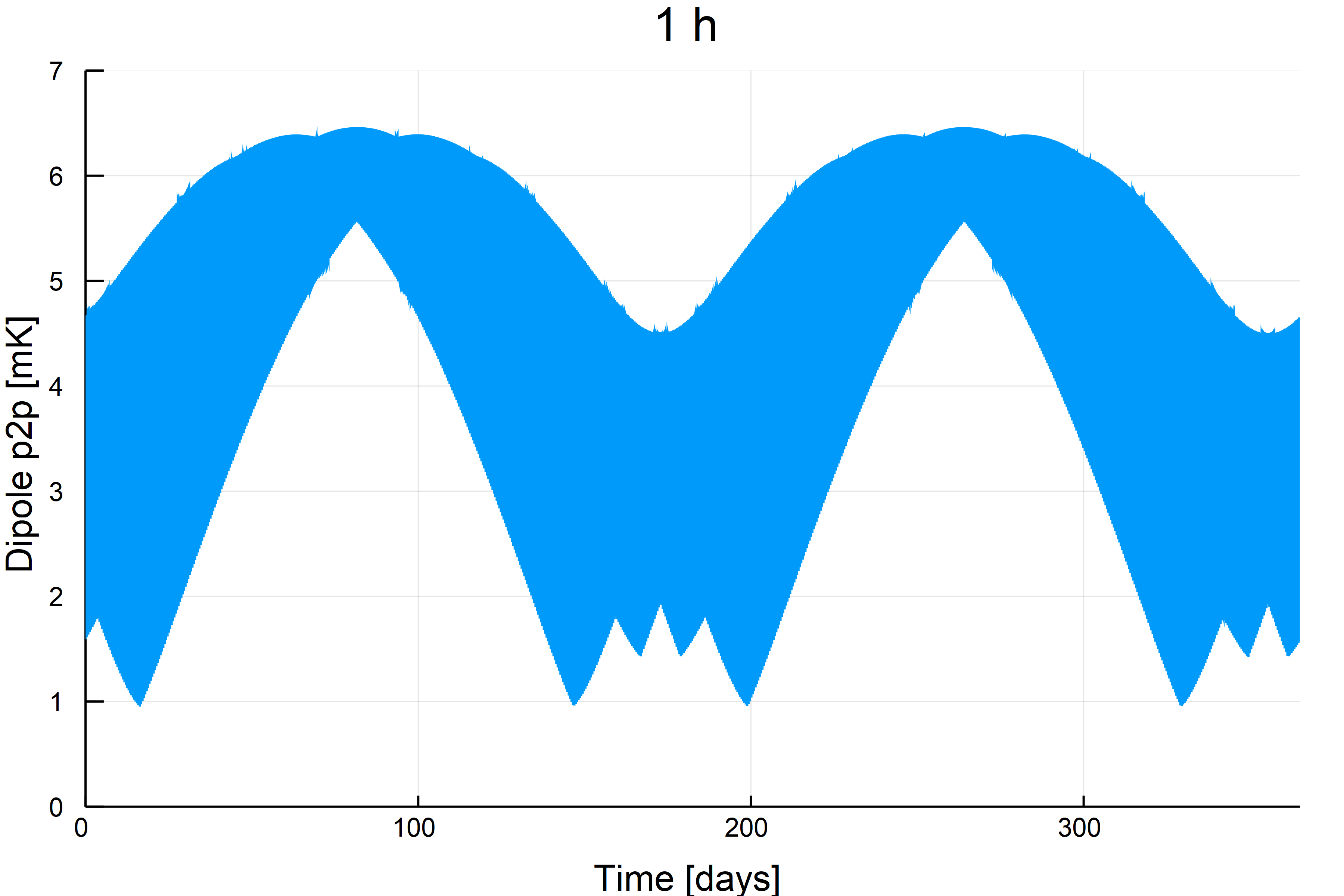
A simple parameter that encapsulates much of the details about photometric calibration is the peak-to-peak variation in the dipole signal during some fixed time span. As PICO detectors are not meant to perform absolute measurements, the modulation of the dipole signal consititutes our calibration source. The peak-to-peak amplitude of the dipole is therefore a good tracer of the S/N for the calibration signal.

Consider this image, which shows the simulated timeline produced by TOAST for one of the W-band detectors (temperature in K as a function of time in seconds, no Galaxy is present):

The low-frequency modulation is due to the dipole signal, while the high-frequency noise is detector noise. As the plot shows ~100 seconds of data, the peak-to-peak variation of the dipole signal within this time frame is less than 3 mK. The following image shows how the peak-to-peak dipole amplitude changes as a function of the time window used to estimate the peak-to-peak value:

(Go to https://zzz.physics.umn.edu/ipsig/_media/dipole-amplitude.gif to see the animation.)

There are several interesting facts that become apparent from the image above. First of all, there are high-frequency fluctuations which disappear for longer time windows. Specifically, as the length of the time window approaches the precession period, high-frequency fluctuations are present no longer. A second interesting fact is that the plot shows low-frequency fluctuations as well. These are unavoidable and are due to the yearly variation in the angle between the spacecraft spin axis and the CMB dipole axis. As a matter of fact, these fluctuations are present even for much longer time windows:

We assume that the calibration code to be used in a real mission would include a component-separation step able to reduce the bias due to the contamination of the dipole signal by Galactic large-scale structures. Therefore, in our simulations we assume that the only signal in the sky apart from the dipole is the CMB itself.

Our simulations assume that each detector has a calibration factor equal to 1.0. The calibration code is therefore expected to retrieve the same value from the simulated data, plus some statistical noise.

I have run a few simulations using DaCapo on the simulated timelines produced by Andrea Zonca. Here are the details:

• 2 years of observation
• 2 boresight W-band detectors
• No Galaxy
• Planck2015 solar dipole, including the quadrupolar correction
• No orbital dipole
• 1/f + WN, with fknee = 10 mHz (corresponding to a period of 100 s).
• Constant gain (1.0)

As DaCapo implements a destriper as well, let's check that the 1/f is correctly estimated. The baseline I used was 10 s:

This plot is complicate to understand due to the presence of the sky signal (the dipole peak and its harmonics). Let's compute the PSD of the noise component alone: this is easy, since TOAST saves the TOD of the foreground signal in a separate column in the FITS files.

The peak at 167 mHz corresponds to the spin period (60 s): note that the height of this residual peak matches the level of the high-frequency WN tail. Apart from that, 1/f is correctly suppressed by the code.

The estimated gains for a time window of 10 hours (the same as the precession period) are shown here:

You can see that the RMS of the gain factors varies with time. This is anticorrelated with the peak-to-peak amplitude of the dipole (see the plot above). The average value of the gains shows some residual bias, as it is not exactly 1.0. The RMS of the timeline is 0.04%, which can be considered as an estimate of the relative calibration error.